【量子力学再入門23】
シュレディンガー方程式の固有状態の数値計算

本稿では、時間に依存しないシュレディンガー方程式の固有状態の数値解を求める方法を解説します。 ポテンシャルが時間に依存しない１次元シュレディンガー方程式は次のとおりです。

\begin{align} -\frac{\hbar^2 }{2m} \frac{d^2 \varphi(x) }{d x^2} +V(x)\varphi(x) = E \varphi(x) \end{align}

この方程式の数値解を得るための方法を示します。通常このような線形波動方程式の数値解は空間差分に境界条件を加えて得ますが、 本稿では時間依存のあるシュレディンガーの数値解を得るための計算法「スペクトル法」との相性を考慮して、波動関数とポテンシャル項の空間依存性をフーリエ変換

\begin{align} \varphi(x) = \sum\limits_{n} a_n \, e^{ik_nx} \ \ , \ \ V(x) =\sum\limits_{l} v_l \, e^{ik_lx} \end{align}

した際の$a_n$を計算します。「スペクトル法」の場合と同様にフーリエ係数$a_n$と$v_l$の関係を導くと

\begin{align} \frac{\hbar^2k_n^2}{2m}\, a_n +\sum\limits_{l} v_l\,a_{n-l} = E\, a_n \end{align}

と得られます。この方程式は$a_0, a_1, a_2,\cdots$に関する連立方程式となっています。この関係式を行列で表したのが次式です。

\begin{align} \left(\matrix{ \epsilon _0+v_0 & v_{-1} & v_{-2} & \cdots \cr v_0 & \epsilon _1+v_{-1} & v_{-2} & \cdots \cr v_0 & v_{-1} & \epsilon _2+v_{-2} & \cdots \cr \vdots & \vdots & \vdots & \ddots } \right) \left(\matrix{ a_0 \cr a_1 \cr a_2 \cr \vdots }\right) = E \left(\matrix{ a_0 \cr a_1 \cr a_2 \cr \vdots }\right) \end{align}

ただし、$\epsilon _n = \hbar^2k_n^2/2m $です。この関係式はシュレディンガー方程式を行列で表した形式になります。$E$と$a_n$と行列

\begin{align} M=\left(\matrix{ \epsilon _0+v_0 & v_{-1} & v_{-2} & \cdots \cr v_0 & \epsilon _1+v_{-1} & v_{-2} & \cdots \cr v_0 & v_{-1} & \epsilon _2+v_{-2} & \cdots \cr \vdots & \vdots & \vdots & \ddots } \right) \end{align}

の固有値と固有ベクトルに対応します。Mの固有値と固有ベクトルを数値計算します。ちなみに$M$は$ M^\dagger =M$を満たすエルミート行列であるため、固有値は必ず実数となります。また、固有値の小さな順に$E_0, E_1, E_2, \cdots$、対応する固有ベクトル（縦ベクトル）を

\begin{align} \boldsymbol a_{0} = \left(\matrix{ a_0^{(0)} \cr a_1^{(0)} \cr a_2^{(0)} \cr \vdots} \right) , \ \boldsymbol a_{1} = \left(\matrix{ a_0^{(1)} \cr a_1^{(1)} \cr a_2^{(1)} \cr \vdots} \right) , \ \boldsymbol a_{2} = \left(\matrix{ a_0^{(2)} \cr a_1^{(2)} \cr a_2^{(2)} \cr \vdots} \right),\cdots \end{align}

と表わし、さらに、固有値を対角に並べた対角行列を

\begin{align} E = \left(\matrix{ E_0 & 0 & 0 & \cdots \cr 0 & E_1& 0 & \cdots \cr 0 & 0 & E_2 & \cdots \cr \vdots & \vdots & \vdots & \ddots } \right) \end{align}

と定義、固有ベクトル（列ベクトル）を横に並べた正方行列を

\begin{align} A=\left( \matrix{ \boldsymbol {a}_{0} & \boldsymbol {a}_{1} & \boldsymbol {a}_{2} & \cdots } \right) \end{align}

と定義すると、$MA=AE \to A^{-1}MA = E$という関係もあります。

調和ポテンシャルの固有状態

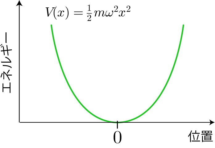
シュレディンガー方程式の数値計算で求める固有状態の妥当性を調べるために、解析解が知られている大きさが距離の２乗に比例する調和ポテンシャルを対象とします。本稿では原点から$10^{-8}[{\rm m}]$離れた際のポテンシャルエネルギーの大きさが$1[{\rm eV}]$となるように$\omega$を与えることにします。

図1 調和ポテンシャルの模式図

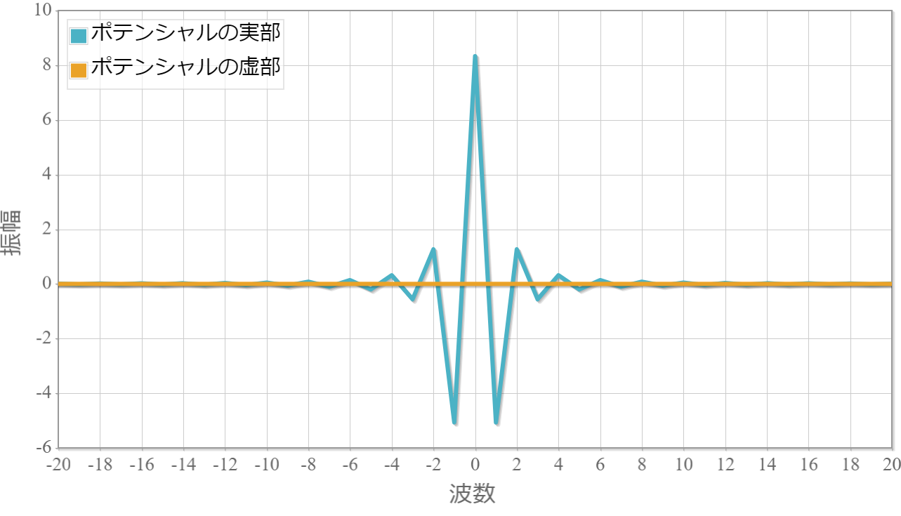
この調和ポテンシャルに対するフーリエ係数（$v_n$）は以下のとおりです。実部と虚部を分けてプロットしています（ $ k_n =2\pi n / L $、$L = 5.0 \times 10^{-8}[{\rm m}]$、$N=1024$ ）。

図2 調和ポテンシャルのフーリエ係数

これで行列$M$の全要素は得られました。エルミート行列$M$の固有値と固有ベクトルをGSLを用いて計算してみましょう。まずは固有値です。調和ポテンシャル項が存在するシュレディンガー方程式の固有値の解析解は

\begin{align} E_n =\, \hbar \omega(n+\frac{1}{2}) \end{align}

と知られているため、これと数値解を比較します。

図3 固有値（固有エネルギー）の解析解と数値解

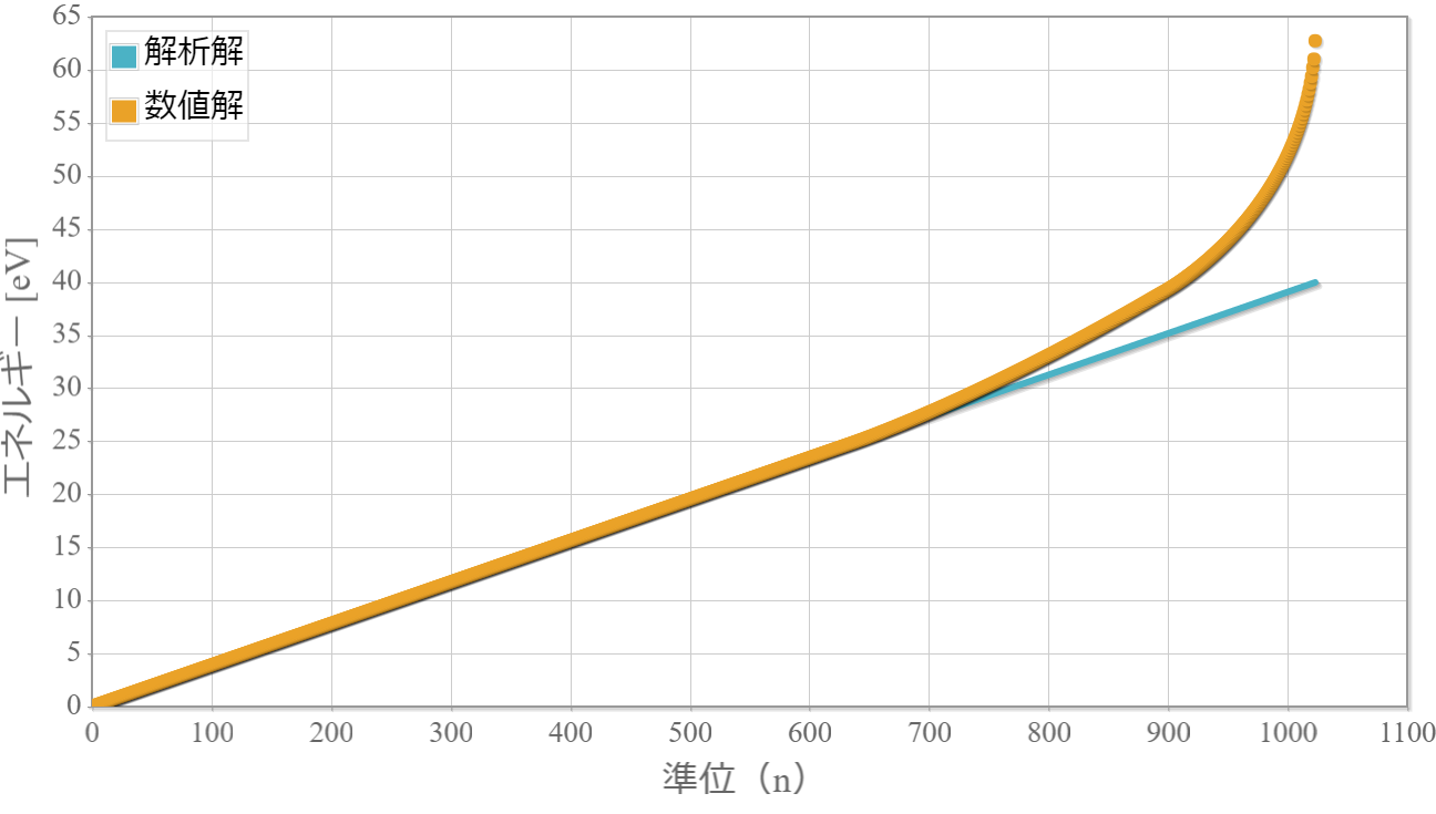
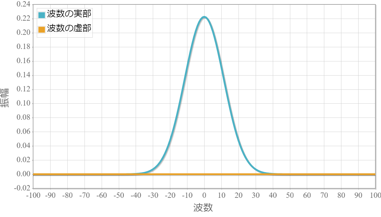
$n$の小さな領域では解析とほぼ一致しますが、大きくなるにつれて解析解とのズレが生じてきます。これはフーリエ変換時の区間Lと項数$N$を大きさに依存します。次のグラフは基底状態（固有値が最小）の$a_n$の実部と虚部です。基底状態は対称なので虚部は０となります。

図4 基底状態（最低固有値に対応する状態）のフーリエ係数の実部と虚部

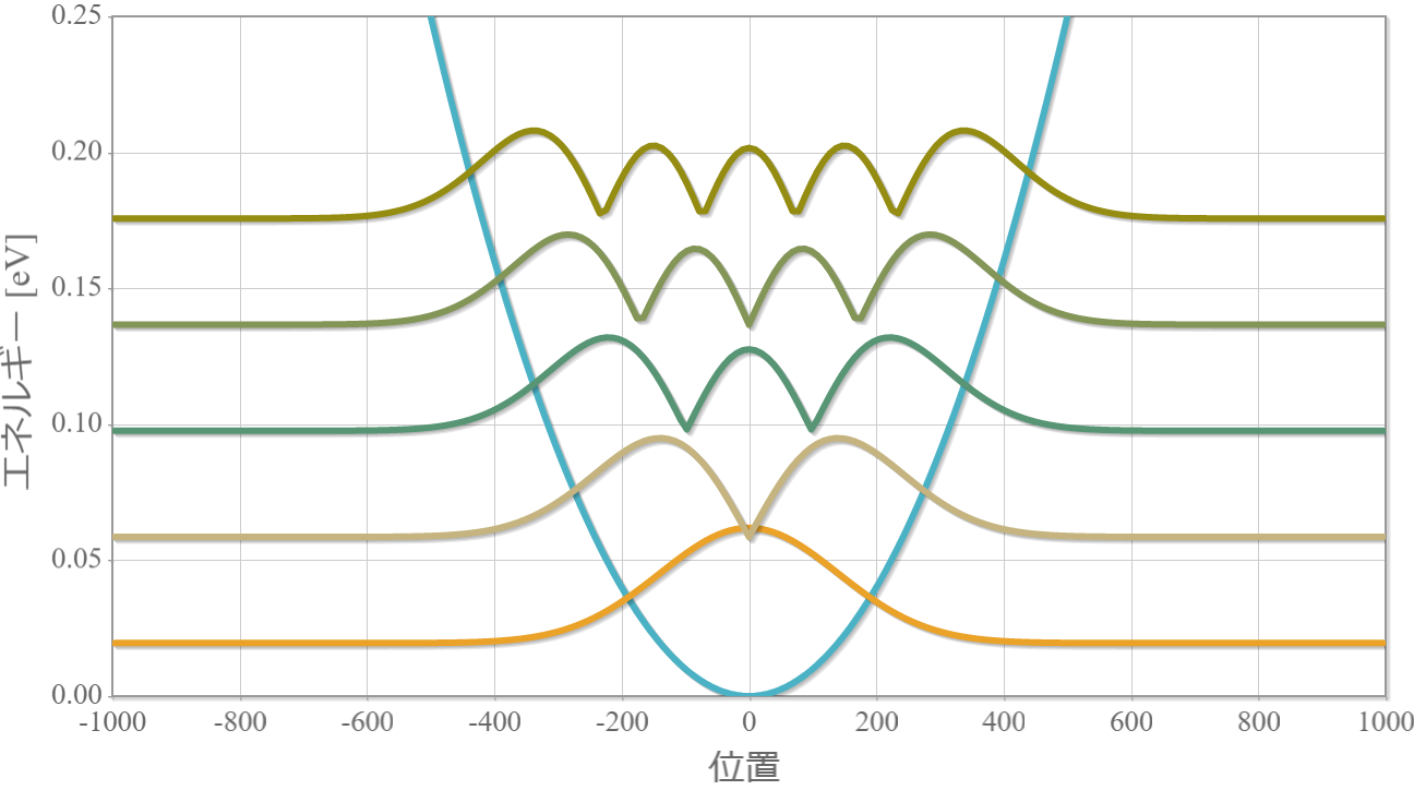
最後に、得らえた$a_n$を逆フーリエ変換して、波動関数の実空間分布を示したのが次の図です。基底状態を含めて下から５つの波動関数を描画しています。各波動関数の振幅０の高さを固有エネルギー（固有値）の値に合わせているので、調和ポテンシャルの空間分布との関係がわかりやすくなっています。

図5 調和ポテンシャルと基底状態から５個の固有状態（実空間分布）

これで任意のポテンシャル項に対する固有状態を計算することができました。次回はスペクトル法と組み合わせて、時間依存性のあるポテンシャルによる励起状態のシミュレーションを行います。

プログラムソース

 

////////////////////////////////////////////////////////////////////
// シュレディンガー方程式の数値計算（調和ポテンシャル中の電子の固有状態）
////////////////////////////////////////////////////////////////////
#define _USE_MATH_DEFINES
#include <math.h>
#include <stdlib.h>
#include <time.h>
#include <memory>
#include <iostream>
#include <fstream>
#include <sstream>
#include <string>
#include <cstdio>
#include <iomanip>
#include <stdio.h>
#include <complex>
#include <omp.h>
#include <direct.h>

#include <gsl/gsl_errno.h>
#include <gsl/gsl_fft_complex.h>
#include <gsl/gsl_math.h>
#include <gsl/gsl_blas.h>
#include <gsl/gsl_vector.h>
#include <gsl/gsl_matrix.h>
#include <gsl/gsl_eigen.h>
#include <gsl/gsl_sort_vector.h>
#include <gsl/gsl_complex.h>
#include <gsl/gsl_complex_math.h>

#define REAL(z,i) ((z)[2*(i)])
#define IMAG(z,i) ((z)[2*(i)+1])
/////////////////////////////////////////////////////////////////
//物理定数
/////////////////////////////////////////////////////////////////
//光速
const double c = 2.99792458E+8;
//真空の透磁率
const double mu0 = 4.0*M_PI*1.0E-7;
//真空の誘電率
const double epsilon0 = 1.0 / (4.0*M_PI*c*c)*1.0E+7;
//プランク定数
const double h = 6.6260896 * 1.0E-34;
double hbar = h / (2.0*M_PI);
//電子の質量
const double me = 9.10938215 * 1.0E-31;
//電子ボルト
const double eV = 1.60217733 * 1.0E-19;
//複素数
const std::complex<double> I(0.0, 1.0);
/////////////////////////////////////////////////////////////////
//物理系の設定
/////////////////////////////////////////////////////////////////
//空間分割サイズ
double dz = 1.0E-11;

//ルンゲクッタ波数の個数（E0=10.eVの場合、Npulseの10倍程度が必要）
const int Ncutoff = 256;
//系のサイズ（周期系）
double L = 5000.0*dz;

//中心エネルギー_波束の重ね合わせ数_時間スケール_FFT分割数
std::string fn = "_HO_2.0_";
//ファイル名
std::string folder = "output";//作成するフォルダ名
std::string filepath1 = folder + "/an" + fn + ".txt";
std::string filepath2 = folder + "/realspace" + fn + ".txt";
std::string filepath3 = folder + "/wavenumber" + fn + ".txt";
std::string filepath4 = folder + "/eigenvalue" + fn + ".txt";

//実空間出力範囲
double x_min = -1000.0*dz;
double x_max = 1000.0*dz;

////ポテンシャル
//double V1 = 10.0 * eV;
//double V2 = 0.0 * eV;
//double V3 = 10.0 * eV;
////量子井戸の幅
//double d = 1000 * dz;
//double V(double x) {
//	if (x <= -d / 2.0) return V1;
//	else if (x <= d / 2.0) return V2;
//	else return V3;
//}

//調和ポテンシャルの定義
double omega = sqrt(2.0 * 1.0 * eV / me) / (1000.0*dz);
double V(double x) {
	return 1.0 / 2.0 * me * omega * omega * x * x;
}


int main() {
	//フォルダ生成
	_mkdir(folder.c_str());

	double v_data[2 * Ncutoff];
	double a_data[2 * Ncutoff];

	std::unique_ptr< double[] > vn_real(new double[Ncutoff]);
	std::unique_ptr< double[] > vn_imag(new double[Ncutoff]);
	std::unique_ptr< double[] > epsilon(new double[Ncutoff]);
	std::unique_ptr< double[] > an_real(new double[Ncutoff]);
	std::unique_ptr< double[] > an_imag(new double[Ncutoff]);
	std::unique_ptr< double[] > energy(new double[Ncutoff]);

	std::unique_ptr< std::complex<double>[][Ncutoff] > an(new std::complex<double>[Ncutoff][Ncutoff]);

	//////////////////////////////////////////////////////////////////////
	// ポテンシャル項のフーリエ変換
	//////////////////////////////////////////////////////////////////////
	for (int n = 0; n < Ncutoff; n++) {
		double x = L / Ncutoff * n;
		if (n < Ncutoff / 2) {
			x = L / Ncutoff * n;
		}
		else {
			x = -L / Ncutoff * (Ncutoff - n);
		}

		REAL(v_data, n) = V(x);
		IMAG(v_data, n) = 0.0;

	}
	//フーリエ変換（順変換）
	gsl_fft_complex_radix2_forward(v_data, 1, Ncutoff);

	//出力ストリームによるファイルオープン
	std::ofstream fout3;
	fout3.open(filepath3.c_str());
	fout3 << "#x:波数" << std::endl;
	fout3 << "#y:振幅" << std::endl;
	fout3 << "#legend: ポテンシャルの実部 ポテンシャルの虚部" << std::endl;
	fout3 << "#showLines: true true true true false false" << std::endl;
	fout3 << "#showMarkers: false false false false true true" << std::endl;
	fout3 << "#fills: false false false false" << std::endl;
	fout3 << "#times:1.0 1.0 1.0 1.0" << std::endl;

	//fout3 << "#xrange:" << -Lz / 2 << " " << Lz / 2 << " " << Lz / 10 << std::endl;
	//fout3 << "#yrange:" << -0.4 << " " << 1 << " " << 0.1 << std::endl;

	for (int n = 0; n < Ncutoff; n++) {

		double kn;
		if (n < Ncutoff / 2) {
			kn = 2.0 * M_PI / L * n;
		}
		else {
			kn = -2.0 * M_PI / L * (Ncutoff - n);
		}
		epsilon[n] = hbar * hbar * kn * kn / (2.0 * me);
		vn_real[n] = REAL(v_data, n) / Ncutoff;
		vn_imag[n] = IMAG(v_data, n) / Ncutoff;

		if (n < Ncutoff / 2) {
			fout3 << n;
		}
		else {
			fout3 << -(Ncutoff - n);
		}

		fout3 << " " << vn_real[n] / eV << " " << vn_imag[n] / eV << std::endl;

	}
	fout3.close();

	//////////////////////////////////////////////////////////////////////
	// エルミート行列の準備
	//////////////////////////////////////////////////////////////////////
	//GSL複素数ベクトルのメモリ確保（固有ベクトル用）
	gsl_vector_complex *eig_vec = gsl_vector_complex_alloc(Ncutoff);
	//GSL複素数ベクトルのメモリ確保（固有値ベクトル用）
	gsl_vector *eig = gsl_vector_alloc(Ncutoff);
	//GSL複素数行列のメモリ確保（エルミート行列用）
	gsl_matrix_complex *matrix = gsl_matrix_complex_alloc(Ncutoff, Ncutoff);
	//GSL複素数行列のメモリ確保（固有ベクトルのまとめ行列用）
	gsl_matrix_complex *eig_vecs = gsl_matrix_complex_alloc(Ncutoff, Ncutoff);
	//エルミート行列の設定
	gsl_matrix_complex *M = gsl_matrix_complex_alloc(Ncutoff, Ncutoff);

	for (int i = 0; i < Ncutoff; i++) {
		for (int j = 0; j < Ncutoff; j++) {
			gsl_complex M_data;

			if (i == j) {
				M_data = {
					epsilon[i] + vn_real[0], //実部
					vn_imag[0] //虚部
				};
			}
			else {
				int l = i - j;
				double sign = (l >= 0) ? 1.0 : -1.0;

				M_data = {
					vn_real[abs(l)], //実部
					vn_imag[abs(l)] * sign  //虚部
				};
			}
			gsl_matrix_complex_set(M, i, j, M_data);
		}
	}

	//////////////////////////////////////////////////////////////////////
	// 固有値と固有ベクトルの計算
	//////////////////////////////////////////////////////////////////////
	// 作業領域の確保
	gsl_eigen_hermv_workspace *workspace_v = gsl_eigen_hermv_alloc(Ncutoff);
	// 行列のコピー
	gsl_matrix_complex_memcpy(matrix, M);
	// 固有値・固有ベクトルの計算
	gsl_eigen_hermv(matrix, eig, eig_vecs, workspace_v);
	//固有ベクトルと固有値の並び替え
	gsl_eigen_hermv_sort(eig, eig_vecs, GSL_EIGEN_SORT_ABS_ASC);
	//数値の昇順 : GSL_EIGEN_SORT_VAL_ASC 
	//数値の降順 : GSL_EIGEN_SORT_VAL_DESC
	//絶対値の昇順 : GSL_EIGEN_SORT_ABS_ASC 
	//絶対値の降順 : GSL_EIGEN_SORT_ABS_ASC 

	//出力ストリームによるファイルオープン
	std::ofstream fout4;
	fout4.open(filepath4.c_str());
	fout4 << "#x:準位（n）" << std::endl;
	fout4 << "#y:エネルギー [eV]" << std::endl;
	fout4 << "#legend: 解析解 数値解" << std::endl;
	fout4 << "#showLines: true false true true false false" << std::endl;
	fout4 << "#showMarkers: false true false false true true" << std::endl;
	fout4 << "#fills: false false false false" << std::endl;


	// 固有値の書き出し
	std::cout << "-----固有値-----" << std::endl;
	for (int n = 0; n < Ncutoff; n++) {
		//解析解
		double En = hbar * omega / 2.0 * (2 * n + 1);
		//固有エネルギー
		energy[n] = gsl_vector_get(eig, n);

		if (n < 10) {
			std::cout << n + 1 << "番目の固有値: " << energy[n] / eV << "  （" << En / eV << "） " << std::endl;
		}

		fout4 << n << " " << En / eV << " " << energy[n] / eV << std::endl;

		for (int j = 0; j < Ncutoff; j++) {
			gsl_complex a_temp = gsl_matrix_complex_get(eig_vecs, j, n);
			an[n][j] = std::complex<double>(GSL_REAL(a_temp), GSL_IMAG(a_temp));
		}

	}
	fout4.close();


	std::cout << std::endl;

	//////////////////////////////////////////////////////////////////////
	// 計算チェック  AX - EX == 0 ?
	//////////////////////////////////////////////////////////////////////
	//固有値による対角ベクトルを準備（matrix）
	for (int i = 0; i < Ncutoff; i++) {
		//実部と虚部
		gsl_complex aa = { gsl_vector_get(eig, i) , 0 };
		for (int j = 0; j < Ncutoff; j++) {
			gsl_matrix_complex_set(matrix, j, i, aa);
		}
	}
	//EXを計算
	gsl_matrix_complex_mul_elements(matrix, eig_vecs);

	gsl_complex al = { 1.0, 0.0 };
	gsl_complex beta = { -1.0, 0.0 };

	//AX-EXを計算
	gsl_blas_zgemm(CblasNoTrans, CblasNoTrans, al, M, eig_vecs, beta, matrix);

	double max = 0;
	for (int i = 0; i < Ncutoff; i++) {
		for (int j = 0; j < Ncutoff; j++) {
			gsl_complex z_temp = gsl_matrix_complex_get(matrix, i, j);
			double abs_z = sqrt(GSL_REAL(z_temp)*GSL_REAL(z_temp) + GSL_IMAG(z_temp)*GSL_IMAG(z_temp));
			if (max < abs_z) max = abs_z;
		}
	}
	std::cout << "検算：AX-XE の要素の最大値 =" << max << std::endl;

	//////////////////////////////////////////////////////////////////////
	// 基底状態の波数
	//////////////////////////////////////////////////////////////////////
	//出力ストリームによるファイルオープン
	std::ofstream fout1;
	fout1.open(filepath1.c_str());
	fout1 << "#x:波数" << std::endl;
	fout1 << "#y:振幅" << std::endl;
	fout1 << "#legend: 波数の実部 波数の虚部" << std::endl;
	fout1 << "#showLines: true true true true false false" << std::endl;
	fout1 << "#showMarkers: false false false false true true" << std::endl;
	fout1 << "#fills: false false false false" << std::endl;
	for (int j = 0; j < Ncutoff; j++) {
		if (j < Ncutoff / 2) {
			fout1 << j;
		}
		else {
			fout1 << -(Ncutoff - j);
		}
		fout1 << " " << an[0][j].real() << " " << an[0][j].imag() << std::endl;
	}
	fout1.close();

	//////////////////////////////////////////////////////////////////////
	// 実空間の波動関数
	//////////////////////////////////////////////////////////////////////
	//出力ストリームによるファイルオープン
	std::ofstream fout2;
	fout2.open(filepath2.c_str());
	fout2 << "#x:位置" << std::endl;
	fout2 << "#y:エネルギー [eV]" << std::endl;
	fout2 << "#showLines: true true true true true true" << std::endl;
	fout2 << "#showMarkers: false false false false false false" << std::endl;
	fout2 << "#fills: false false false false" << std::endl;
	fout2 << "#fills: false false false false" << std::endl;
	fout2 << "#yrange:0 0.3 0.05"  << std::endl;

	for (int j = 0; j < Ncutoff; j++) {
		REAL(v_data, j) = vn_real[j];
		IMAG(v_data, j) = vn_imag[j];
	}
	gsl_fft_complex_radix2_backward(v_data, 1, Ncutoff);

	fout2 << "#dataset: 0" << std::endl;
	//ポテンシャルの実空間分布
	for (int n = 0; n < Ncutoff; n++) {
		double x;
		if (n < Ncutoff / 2) x = L / Ncutoff * n;
		else x = -L / Ncutoff * (Ncutoff - n);
		if (x < x_min || x_max < x) continue;

		fout2 << x / dz<< " " << REAL(v_data, n) / eV <<  std::endl;
	}

	for (int i = 0; i < 5; i++) {
		fout2 << "#dataset: "<< i + 1 << std::endl;

		for (int j = 0; j < Ncutoff; j++) {
			REAL(a_data, j) = an[i][j].real();
			IMAG(a_data, j) = an[i][j].imag();
		}

		//逆変換の実行
		gsl_fft_complex_radix2_backward(a_data, 1, Ncutoff);

		for (int n = 0; n < Ncutoff; n++) {
			double x = L / Ncutoff * n;
			if (n < Ncutoff / 2) {
				x = L / Ncutoff * n;
			}
			else {
				x = -L / Ncutoff * (Ncutoff - n);
			}

			if (x < x_min || x_max < x) continue;

			double absPhi = sqrt(REAL(a_data, n)*REAL(a_data, n) + IMAG(a_data, n)*IMAG(a_data, n)) / 150;

			fout2 << x / dz << " " << absPhi + energy[i]/eV <<  std::endl;
		}

	}

	fout2.close();

	//領域の開放
	gsl_matrix_complex_free(eig_vecs);
	gsl_eigen_hermv_free(workspace_v);
	gsl_matrix_complex_free(M);
	gsl_matrix_complex_free(matrix);
	gsl_vector_complex_free(eig_vec);
	gsl_vector_free(eig);


	std::cout << "finished" << std::endl;


	int a;
	std::cin >> a;
	return a;

}

参考ページ

・スペクトル法による波動関数の時間発展の計算方法
・GNU科学技術計算ライブラリ（GSL）について
・GSLによる高速フーリエ変換（FFT）
・GSLによるエルミート行列の固有値・固有ベクトルの計算
・１次元量子力学における調和振動子